|
Objective and Overview
The objective of this tutorial is to
learn how to use the MMTSB Tool Set for carrying out and analyzing simulations with CHARMM.
|
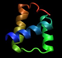
In this tutorial the engrailed homeodomain from Drosophila melanogaster is used as an example. A crystal structure
is available from the Protein Data Bank
with the PDB code
1ENH. A picture is shown on the right.
|
|
1. Initial Structure
Begin by downloading/copying the PDB file for the engrailed homeodomain (1ENH). Extract the protein
atoms from the PDB file with:
convpdb.pl -nsel protein 1ENH.pdb > 1enh.protein.pdb
In this structure hydrogens are still missing. Because the all-atom force field we will
be using needs all atoms including hydrogens we need to add them. This can
be done with complete.pl:
complete.pl 1enh.protein.pdb > 1enh.protein.allh.pdb
Check the result and verify that the structure is indeed complete now. This
tool will also help adding missing atoms, however, it cannot add missing
residues.
2. Energy Minimization
Before we can run any simulation we have to minimize the protein conformation.
As a somewhat realistic but very fast method for representing aqueous solvent
we will use a distance dependent dielectric function with an epsilon value of 4.
We will also use restraints on the C-alpha coordinates in order to preserve the
overall shape of the initial structure:
    minCHARMM.pl -par dielec=rdie,epsilon=4,minsteps=50 \
                 -cons ca self 3:56_1.0 -log min.log \
                  1enh.protein.allh.pdb > 1enh.min.pdb
This script will carry out steepest descent minimization first and then a more effective
minimization method (Adopted-Basis Newton-Raphson) over 50 steps. The result is normally
written to standard output, so we need to redirect it into a file.
Take a look at the CHARMM output in the file min.log and see how the
energy decreases rapidly during the minimization run.
The minimized structure can now be used to start a molecular dynamics simulation.
3. Explicit Solvent Simulation
Next, we will setup a simulation box for an explicit solvent simulation.
First, we need to solvate our protein in a box of water:
convpdb.pl -solvate -cubic -cutoff 9 1enh.min.pdb > 1enh.solvated.pdb
This command generates a cubic box of waters around the protein so that there are at least
9 Angstroms (~3 water layers) between the protein and the edge of the box. If you use a
smaller cutoff you risk periodic artifacts, with a larger cutoff the simulation will quickly
become much more expensive. Write down the size of the box from the output and take a look
at the resulting file with VMD. Nice water box, isn't it?
We are almost ready to start the simulation, but with explicit solvent we also need to
think about ions. First, let's check what the charge of the protein is:
enerCHARMM.pl -charge 1enh.min.pdb
You should find that the engrailed homeodomain has a charge of +7. Therefore, we need to
add 7 negatively charged counterions. We will use chlorine ions that can be added
by replacing water molecules randomly with the following command:
convpdb.pl -ions CLA:7 1enh.solvated.pdb > 1enh.waterions.pdb
Let's check the charge of the entire sytem again:
enerCHARMM.pl -charge 1enh.waterions.pdb
If the result is not zero, something went wrong.
We will now minimize the entire simulation box again (fill in the actual boxsize
instead of xxx):
minCHARMM.pl -par minsteps=50,boxsize=xxx 1enh.waterions.pdb > 1enh.wations.min.pdb
We start the simulation by heating the system slowly. Three simulations
at 100K, 250K, and then 300K are enough for this exercise, but in other cases a longer
equilibration protocol may be needed. These steps while take a little while to complete:
  mdCHARMM.pl -par dynsteps=250,boxsize=xxx,dyntemp=100 -final xplicit.md1.pdb 1enh.wations.min.pdb
  mdCHARMM.pl -par dynsteps=250,boxsize=xxx,dyntemp=250 -final xplicit.md2.pdb xplicit.md1.pdb
  mdCHARMM.pl -par dynsteps=250,boxsize=xxx,dyntemp=300 -final xplicit.md3.pdb xplicit.md2.pdb
Now we are ready to run a longer simulation at 300K that we will analyze afterwards:
  mdCHARMM.pl -par dynsteps=2000,boxsize=xxx,dyntemp=300,dynoutfrq=10 \
              -cmd md.cmd -log xplicit.md4.log -trajout xplicit.md4.dcd \
              -final xplicit.md4.pdb xplicit.md3.pdb &
The additional options are used to
generate a log file and a trajectory file with conformations saved
every 10 steps (dynoutfrq parameter).
These commands seem very
simple, but the Tool Set is taking care of quite a few of the setup
tasks needed to run explicit solvent simulations with CHARMM. You may
take a look at the file 'md.cmd' to see what commands are actually sent
to CHARMM in order to run the simulation. The '&' at the end of the
command will run the command in the background so that we can continue
with the next step of this tutorial while the explicit solvent
simulation is running. 4. Implicit Solvent Simulation
It is easier to run an implicit solvent simulation than with explicit solvent.
We do not need to generate a solvent box. Starting from the minimized protein structure
we will follow the same equilibration protocol as for explicit solvent:
    mdCHARMM.pl -par gb,dynsteps=250,dyntemp=100 -final impl.md1.pdb 1enh.min.pdb
    mdCHARMM.pl -par gb,dynsteps=250,dyntemp=250 -final impl.md2.pdb impl.md1.pdb
    mdCHARMM.pl -par gb,dynsteps=250,dyntemp=300 -final impl.md3.pdb impl.md2.pdb
The flag 'gb' selects the GBMV
generalized Born implicit solvent method. After the initial
equilibration we are ready to also run a longer run with the GB method.
For the production run we will turn on Langevin dynamics with a
friction coefficient of 10/ps in order to obtain realistic interactions
with the solvent:
  mdCHARMM.pl -par gb,dynsteps=2000,dyntemp=300,dynoutfrq=10,lang,langfbeta=10 \
              -cmd md.cmd -log impl.md4.log -trajout impl.md4.dcd \
              -final impl.md4.pdb impl.md3.pdb &
Wait until both the explicit and implicit solvent simulations are finished.
5. Analysis
There are many ways in which a molecular dynamics trajectory can be analyzed.
First, load the final PDB and the DCD files into VMD to animate the trajectories.
Second, the MMTSB Tool Set offers
the utility analyzeCHARMM.pl to carry out quantitative analysis functions through CHARMM.
We will begin by calculating the root mean square deviation of the simulated engrailed homeodomain from
the initial minimized structure as a function of time in both the explicit and implicit solvent
simulations:
  analyzeCHARMM.pl -rms -sel CA -comp 1enh.min.pdb \
                   -pdb xplicit.md4.pdb xplicit.md4.dcd > xplicit.rmsd
  analyzeCHARMM.pl -rms -sel CA -comp 1enh.min.pdb \
                   -pdb impl.md4.pdb impl.md4.dcd > implicit.rmsd
The analysis command reads a DCD output file, but also requires a matching PDB to describe the system.
The reference structure for the RMSD calculation is given with the -comp option. Which
atoms are used for the RMSD calculation can be specified with -sel, in this example C-alpha
atoms were chosen.
Plot both curves and compare them. What do you find?
Next, we will calculate the radial density profile of water oxygens with respect to the center of
mass of the solute. Such profiles are useful to check whether the number density at the edge of the
box approaches the correct bulk solvent density of 0.03337 waters/A^3.
  analyzeCHARMM.pl -rdist -ndens -cofm -dsel water.OH2 solute \
                   -par boxsize=xxx -pdb xplicit.md4.pdb xplicit.md4.dcd > radial.profile
Last, phi/psi dihedral angles can be calculated with the following command:
analyzeCHARMM.pl -sel <resno> -phi -psi -pdb impl.md4.pdb impl.md4.dcd
Use that command to find a residue where the phi/psi angle varies significantly
over the course of the (very short) simulations and plot the trajectory in a
phi/psi plot.
|