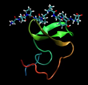
This tutorial will explore the ensemble computing capabilities of the MMTSB Tool Set. As an example the WW domain from Yes-associated protein (Yap), for which a structure has been reported in complex with a bound proline rich peptide is used to estimate the binding energy using molecular dynamics and MM/GB binding energy estimates.


This tutorial will illustrate how we can use the MMTSB Tool Set to run an MD simulation of the protein-ligand complex, create an ensemble structure from this dynamics trajectory and then use the ensemble analysis tools in the MMTSB Tools Set to calculate an approximate binding energy.

Binding energies will be estimated following the MMPB/SA or MMGB/SA scheme. From the conformations sampled during a molecular dynamics simulation of the complex average energies are calculated separately for the complex, the receptor, and the substrate. The binding energy can then be estimated from the difference:

ΔΔG(binding) = ΔG(complex) - ΔG(receptor) - ΔG(ligand)

1. Initial system setup

Obtain/copy the experimental structure of the YAP-WW-domain from the Protein Data Bank. The PDB code is 1JMQ

Because the structure was solved by NMR spectroscopy there are multiple models in the PDB file. Extract the first model with:

    convpdb.pl -model 1 1JMQ.pdb > yapww.pdb
    

Next, we will minimize the experimental structure with distance dependent dielectric as a fast approximation of the solvent environment:

    minCHARMM.pl -par dielec=rdie,epsilon=4,minsteps=50 \
                 -log min.log yapww.pdb > yapww.min.pdb
    

We are now ready to run a molecular dynamics simulation of the complex to obtain conformational samples for the MMGB/SA analysis. Because no explicit solvent is present, the simulation will be run with GB (GBMV). Also, this simulation is very short for this type of analysis, but it will suffice for the purposes of this tutorial.

    mdCHARMM.pl -par dynsteps=2000,dynoutfrq=100 -trajout yapww.dcd \
                -log dynamics.log -final yapww.md.pdb yapww.min.pdb
    

For the subsequent analysis we will take advantage of the ensemble computing facility in the MMTSB Tool Set. In order to use the ensemble computing tools we have to first generate an ensemble directory structure from the trajectory file. This can be done with the following command:

    processDCD.pl -ensdir ens -ens complex yapww.md.pdb yapww.dcd
    

In this case the ensemble data is stored in a subdirectory 'ens' and the conformations from the trajectory are available through the 'complex' tag.

Next, we will extract the substrate (chain P) and receptor (chain A) for each complex into separate files for later analysis:

    ensrun.pl -dir ens -new substrate complex convpdb.pl -chain P
    ensrun.pl -dir ens -new receptor complex convpdb.pl -chain A
    

We now have three files for each snapshot, complex.pdb, receptor.pdb, and substrate.pdb. You should find these files in any of the ensemble subdirectories. You will see, however, that the files are automatically compressed to preserve space.

We are now ready to evaluate the energies that we need for the binding free energy estimate. First, we calculate the total energy for the complex:

    ensrun.pl -dir ens -set dgcomplex:1 complex enerCHARMM.pl \
              -par gb,nocut complex.pdb
    

Second, we will estimate the energies for the substrate and receptor alone:

    ensrun.pl -dir ens -set dgreceptor:1 complex enerCHARMM.pl \
              -par gb,nocut receptor.pdb
    ensrun.pl -dir ens -set dgsubstrate:1 complex enerCHARMM.pl \
              -par gb,nocut substrate.pdb
    

We can take a look at the results with getprop.pl:

    getprop.pl -dir ens -prop dgcomplex,dgreceptor,dgsubstrate complex
    

... or combine results to get the binding free energy for each snapshot

    getprop.pl -dir ens -prop dgcomplex-dgreceptor-dgsubstrate complex
    

... or obtain the average value:

    getprop.pl -dir ens -score avg \
               -prop dgcomplex-dgreceptor-dgsubstrate complex 
    

The result is likely around -30 kcal/mol. That number seems fairly large, but in our analysis so far we have neglected entropic effects related to the substrate and receptor (the entropic effects of the solvent are included in the implicit solvent model).