CTBP SUMMER SCHOOL 2009
A Coupled Potential QM/MM Simulation
By Ross Walker
With the version 9 release of AMBER came the ability to do fast and accurate coupled potential semi-empirical QM/MM simulations with full treatment of long range electrostatics (PME) or Generalized Born implicit solvent simulations. This tutorial uses the theory described section 3.5 of the AMBER 10 manual in which one part of the system can be represented quantum mechanically while the rest of the system is represented using the classical AMBER force field.
This tutorial covers how to set up a periodic boundary QM/MM simulation using AMBER 10. The functionality described here will shortly be integrated into CHARMM with similar functionality.
1) Setting up NMA
In this tutorial we will run two simulations and compare them. In the first simulation we will run a classical MD simulation of N-methylacetamide (NMA) in a periodic box of TIP3P water. In the second simulation we will run the same thing but this time we will use the semi-empirical PM3 Hamiltonian to calculate the energy and force on the NMA molecule.
The first stage is to build a topology and coordinate file for NMA in TIP3P water. NMA is simply an ACE and an NME residue joined together. As such it's structure is simple enough that we don't need to bother obtaining an initial pdb structure. We can simply use the sequence command in LEaP to do it for us. (First download an updated version of xleap, and move it to /opt/bin/amber11/bin.)
$AMBERHOME/exe/xleap -f $AMBERHOME/dat/leap/cmd/leaprc.ff99SB
> NMA = sequence { ACE NME }
Ok, now we have a reasonable structure we can go ahead and add our solvent box. First close the unit editor (Unit->Close). Now we add a solvent box of 15 angstroms around the center of our NMA unit.
solvatebox NMA TIP3PBOX 15
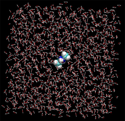
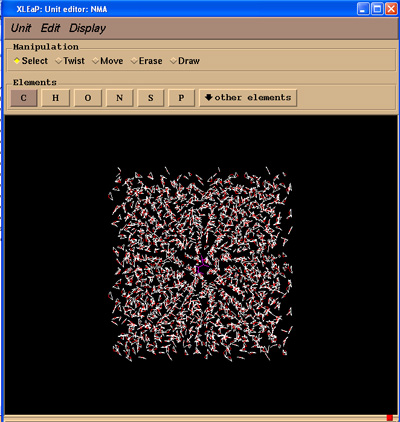
Xleap should report that it added around 1500 residues. If we edit the NMA unit we should now see our solvent box.
edit NMA
Now we can go ahead and save our topology and coordinate files. There is no need to charge neutralise our system since our NMA unit is neutral.
saveamberparm NMA NMA.prmtop NMA.inpcrd
Here are the files: NMA.prmtop NMA.inpcrd
2) Classical MD
Now we have the topology and coordinate files we are ready to carry out classical MD. First things first though we need to minimize our system to remove any bad contacts created by solvation and also to allow our artificially created NMA structure to relax. For this we will run 500 steps of minimization. Here is the input file:
| Initial minimisation of our structure &cntrl imin=1, maxcyc=500, ncyc=200, cut=8.0, ntb=1, ntc=2, ntf=2 / |
$AMBERHOME/exe/sander -O -i min_classical.in -o min_classical.out -p NMA.prmtop -c NMA.inpcrd -r min_classical.rst
Input Files:
min_classical.in,
NMA.prmtop, NMA.inpcrd
Output Files: min_classical.out,
min_classical.rst
Once we have minimized the system we will run 1ps of MD at a constant temperature of 300K. Here is the input file for the MD run:
| 300K constant temp MD &cntrl imin=0, ntb=1, cut=8.0, ntc=2, ntf=2, tempi=300.0, temp0=300.0, ntt=3, gamma_ln=1.0, nstlim=1000, dt=0.002, ntpr=1, ntwx=1, / |
Now we run the md.
$AMBERHOME/exe/sander -O -i md_classical.in -o md_classical.out -p NMA.prmtop -c min_classical.rst -r md_classical.rst -x md_classical.mdcrd
This should take about 3 mins to run.
Input Files: md_classical.in,
NMA.prmtop,
min_classical.rst
Output Files: md_classical.out,
md_classical.rst,
md_classical.mdcrd
Now, let's do two things. First we will visualize our MD trajectory in VMD and secondly we will use ptraj to create an average structure for us.
Step 1 - VMD. Fire up VMD and load the NMA topology file and then load the md_classical.mdcrd file into this molecule. I gzipped it to save space on the webserver so make sure you decompress it first.
While it is good to see our big box of water "floating" about we are more interested in the dynamics of the NMA residue so let's remove the water.
Graphics->Representations
In Selected Atoms type:
all not water
And hit apply
At the same time change the drawing method to CPK.
You should now be able to watch a movie of our NMA molecule "wiggling" about.
The thing to notice is how planar the amide C-N-H group remains during the simulation.
Let's try repeating the simulation using a coupled QM/MM potential.
3) QM/MM MD
We will model the NMA molecule using the semiempirical PM3 Hamiltonian while all the water we will model classically. In this situation we have no bonds crossing the QM/MM boundary and so do not need to worry about where sander will place hydrogen link atoms. However, if we did have bonds that crossed the boundary sander would add the link atoms completely automatically. See the manual for more info.
For QM/MM MD the input files look very similar. There are a few notable differences, however, related to the specification of the atoms to be modeled quantum mechanically. Here is the minimization input file we will use:
|
Initial min of our structure QMMM &cntrl imin=1, maxcyc=500, ncyc=200, cut=8.0, ntb=1, ntc=2, ntf=2, ifqnt=1 / &qmmm qmmask=':1-2', qmcharge=0, qm_theory='PM3', qmshake=1, qm_ewald=1, qm_pme=1 / |
The extra variables in this file are:
ifqnt = 1 - This is the flag that tells sander that we want a QMMM run. It will then look for a &qmmm namelist.
Most of the options specified in the &qmmm namelist are the defaults but it is often good to include them in the input file to make it easier to work out what you did at the later date:
qmmask = ':1-2' - This specifies what to treat quantum mechanically using standard AMBER mask notation. Here it implies residue 1 and 2 which is the ACE and NME making up the NMA molecule. Alternatively you can manually specify the atom numbers using iqmatoms. E.g. iqmatoms=1,2,3,4,5,6,7,8,9,10,11,12,
qmcharge = 0 - The integer charge of the QM region (default = 0)
qm_theory = 'PM3' - Use the PM3 Hamiltonian (default = 1)
qmshake = 1 - Shake QM hydrogen atoms (default = 1 if ntc=2)
qm_ewald = 1 - Use an Ewald type treatment for long range electrostatics (default = 1 if ntb>0)
qm_pme = 1 - Use a Particle Mesh Ewald method as Ewald type (default = 1 if qm_ewald=1 and use_pme=1)
$AMBERHOME/exe/sander -O -i min_qmmm.in -o min_qmmm.out -p NMA.prmtop -c NMA.inpcrd -r min_qmmm.rst
Input Files:
min_qmmm.in,
NMA.prmtop, NMA.inpcrd
Output Files: min_qmmm.out,
min_qmmm.rst
As we did in the classical simulation above we will run 1ps of simulation. Again our input file is the same apart from the QM specifications. Here is the MD input file:
| 300K constant temp QMMMMD &cntrl imin=0, ntb=1 cut=8.0, ntc=2, ntf=2, tempi=300.0, temp0=300.0, ntt=3, gamma_ln=1.0, nstlim=1000, dt=0.002, ntpr=1, ntwx=1,ifqnt=1 / &qmmm qmmask=':1-2', qmcharge=0, qm_theory='PM3', qmshake=1, qm_ewald=1, qm_pme=1 / |
$AMBERHOME/exe/sander -O -i md_qmmm.in -o md_qmmm.out -p NMA.prmtop -c min_qmmm.rst -r md_qmmm.rst -x md_qmmm.mdcrd
You can track the output in another terminal window with "tail -f md_qmmm.out" if you wish. The first thing you should notice with this simulation is that each step takes slightly longer than the classical simulation. The reason for this is that we are doing a complete SCF at every step. However, the difference here should not be huge. This should take around 3 minutes or so to run.
Input Files:
md_qmmm.in,
NMA.prmtop, min_qmmm.rst
Output Files: md_qmmm.out,
md_qmmm.rst, md_qmmm.mdcrd
Take a quick look at the md_qmmm.mdcrd file in VMD to check everything went okay. Remember to gunzip it first.
The final step is to compare the two simulations.
4) Comparing the results
We will now qualitatively compare the results of the two simulations. First of all lets take a brief look at the two output files:
|
Classical |
 NSTEP =        0   TIME(PS) =       0.000  TEMP(K) =   455.28  PRESS =     0.0
 Etot   =     -9086.7258  EKtot   =      4144.0991  EPtot      =    -13230.8249
 BOND   =         0.0650  ANGLE   =         0.1616  DIHED      =         2.5068
 1-4 NB =         1.1157  1-4 EEL =       -19.4429  VDWAALS    =       930.8446
 EELEC  =    -14146.0758  EHBOND  =         0.0000  RESTRAINT  =         0.0000
 Ewald error estimate:   0.1330E-03
 ------------------------------------------------------------------------------
NSTEP = 1 TIME(PS) = 0.002 TEMP(K) = 346.22 PRESS = 0.0 Etot = -10079.4435 EKtot = 3151.3814 EPtot = -13230.8249 BOND = 0.0650 ANGLE = 0.1616 DIHED = 2.5068 1-4 NB = 1.1157 1-4 EEL = -19.4429 VDWAALS = 930.8446 EELEC = -14146.0758 EHBOND = 0.0000 RESTRAINT = 0.0000 Ewald error estimate: 0.1330E-03 ------------------------------------------------------------------------------ |
|
QMMM |
 NSTEP =        0   TIME(PS) =       0.000  TEMP(K) =   455.28  PRESS =     0.0
 Etot   =     -9041.3222  EKtot   =      4144.0991  EPtot      =    -13185.4213
 BOND   =         0.0000  ANGLE   =         0.0000  DIHED      =         0.0000
 1-4 NB =         0.0000  1-4 EEL =         0.0000  VDWAALS    =       881.6951
 EELEC  =    -14012.9122  EHBOND  =         0.0000  RESTRAINT  =         0.0000
 PM3ESCF=       -54.2042
 Ewald error estimate:   0.5641E-01
 ------------------------------------------------------------------------------
NSTEP = 1 TIME(PS) = 0.002 TEMP(K) = 346.23 PRESS = 0.0 Etot = -10033.9525 EKtot = 3151.4687 EPtot = -13185.4213 BOND = 0.0000 ANGLE = 0.0000 DIHED = 0.0000 1-4 NB = 0.0000 1-4 EEL = 0.0000 VDWAALS = 881.6951 EELEC = -14012.9122 EHBOND = 0.0000 RESTRAINT = 0.0000 PM3ESCF= -54.2042 Ewald error estimate: 0.5641E-01 ------------------------------------------------------------------------------ |
The first thing you should notice is that the QM/MM result has an extra field (PM3ESCF). This is the energy due to the quantum part of the calculation (the NMA) within the presence of the charge field of the MM part (the water). You should also notice here that the QM/MM result lacks ANGLE, DIHEDRAL, 1-4 NB and 1-4 EEL energies. This is exactly as we expect since the NMA bonds, angles, dihedrals and VDW and electrostatic terms are now dealt with inside the QM calculation. The only atoms remaining in the MM section are TIP3P water molecules. These are actually triangulated water and so only have bond terms (TIP3P water does not have an angle component). The water molecules are also only 3 atoms in size and so do not have any 1-4 NB or 1-4 EEL interactions.
If you compare the two output files further you should find that the temperatures are reasonably stable and similar. They will not be exactly the same since we are tracking different trajectories.
Now, lets compare the actual dynamics. First off lets load the QM/MM mdcrd file into vmd:
Fire up VMD and load the NMA topology fileand then load the md_qmmm.mdcrd file into this molecule..
We should again remove the water molecules so our NMA is easier to see.
Graphics->Representations
In Selected Atoms type:
all not water
And hit apply
At the same time change the drawing method to CPK.
You should now be able to watch a movie of our NMA molecule "wiggling" about. How does the dynamics of the NMA differ from the classical simulation? If you want you can load both molecules into VMD and animate them together.
Rewind the current QM/MM loaded trajectory to the beginning and then load a new molecule. Select the NMA.prmtop again and then load the md_classical.mdcrd file into this molecule. When you close the load molecule dialog box you should find that both molecules are displayed. You can now play through the trajectory slowly and watch the difference. (You can colour the two molecules differently in Graphics->Representations if you want).
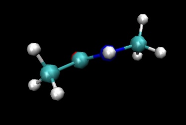
You should notice that the dynamics of the NH group are different in the QM/MM calculation. The nitrogen regularly forms a pyramidal structure and the amine hydrogen is more often out of the O-C-N plane. The QM/MM behaviour here is believed to be the more accurate. The NH backbone dynamics are known to be troublesome to model accurately with classical force fields.
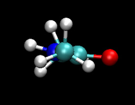 |
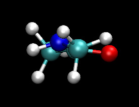 |
| Classical (MM) | QM |
I leave it to you the reader to try other forms of analysis, you could look at the difference between average structures, plot the O-C-N-H out of plane angle as a function of time. You could also try cluster analysis and hydrogen bond analysis. How does the frequency of hydrogen bonds differ between the classical and the QM/MM simulation?
If you want to take this further you could try setting up some more complex systems with QM/MM. A very good system to try is Chorismate Mutase.
(Note: These tutorials are meant to provide
illustrative examples of how to use the AMBER software suite to carry out
simulations that can be run on a simple workstation in a reasonable period of
time. They do not necessarily provide the optimal choice of parameters or
methods for the particular application area.)
Copyright Ross Walker 2009