Solvation with various methods
In order to model a solvated system, approximations must be made to
keep the computation feasible. The best simulation would be as close
to reality as possible. Real systems have orders of magnitude more interactions
to consider than we can realistically compute at present. We choose the
least expensive method of mimicing reality that does not introduce
unacceptable errors into the proprerties that we are trying to model and
study. It is generally accepted that the best way to model a macromolecule
in solution is to surround it with explicit water molecules.
-
Constant dielectric
Vacuum (dielec=1) or constant dielectric medium for small molecules.
-
Distant-dependent dielectric
Crude approximation to solvated system, dielectric increases
from 1 for nearby charge interactions to the specified
dielectric constant for longer range interactions that would
be shielded by the dielectric medium
-
Generalized Born (GB) model
Modified Born equation for solvation energetics. Models solvation
well, with the unrealistic but often desirable instantaneous
response of the implicit solvent yto namics and configuration
echo -n "converting pdb water cube"
of the solute.
-
Explicit water
|
This is the most expensive but best solvation model. One
would place enough water molecules so that wherever the
boundaries of the simulation are, the boundary effects do not
interfere with the energetics and dynamics of the system in a
way that reduces the validity of the properties one is
studying. Enough water is placed around the solute to extend
as far as the cutoff that is used in the nonbonded
interaction determination.
Normally one uses periodic boundary conditions
(PBC) with this type of solvated model in order to
model an infinite solvated system without edge effects
where the water meets the edge of the box. PBC are usually
either cubic or truncated octahedral in shape:
|
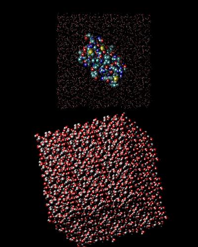
Cubic Boundary explicit water solvated system
5726 water molecules for 10 Å cutoff |
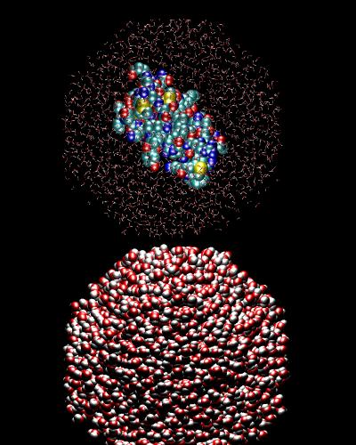
Truncated Octahedron Boundary explicit water solvated system
2844 water molecules for 10 Å cutoff |
 |
 |
Solvation tutorial
(download)
The purpose of this tutorial is to show how to set up a solvated
protein for simulations in which explicit solvent is desired.
First, the simpler methods are demonstrated, constant dielectric, distance
dependent dielectric, and generalized born.
Second, two solvent boxes are created around the protein: cubic and
truncated octahedral. Before these systems can be used to simulate
the system, they need to be equilibrated to relax the high-energy and
unlikely positions of atoms that are due to the construction of the
box of water. This is accomplished by mininizing the system to
remove the high-energy conditions, and equilibrating at constant
tempr
temperature and pressure until the system stabilizes. For this tutorial,
we will not equilibrate for a long enough time to reach a stable system.
One can download the script, change to
to be executable, and execute it
OR
enter each command individually from the shell prompt.