The objective of this tutorial is to illustrate the continuous constant pH molecular dynamics (CPHMD) simulation technique. We will learn to set up CPHMD simulations using the single-temperature or replica-exchange (REX) protocol; analyze the titration data and compute pKa's; obtain parameters for the potential of mean force (PMF) of model compound titration. The C-peptide from ribonuclease A (RNase A) will be used as an example.

1. Prepare a structure with dummy hydrogen atoms

In the CPHMD method, protonation/deprotonation events are modeled by smoothly turning on/off electrostatic and van der Waals interactions involving titratable hydrogen atoms without breaking/forming bonds. Thus, titratable hydrogen atoms can be considered as dummy atoms that are covalently attached during the entire simulation time. To enable double-site titration for carboxyl groups, we attach dummy hydrogen atoms to
both carboxylate oxygens.

First, we extract the first 13 residues from RNase A (PDB ID: 1RNU) and convert the PDB file to the CHARMM format. Remember to replace the residue name HSD with HSP so we can titrate both d- and e- protons in His.

convpdb.pl -sel 1:13 -out charmm22 -segnames 1RNU.pdb | sed "s/HSD/HSP/g" > cpept.pdb

Next, we add dummy hydrogen atoms to the carboxyl residues (Asp and Glu) using patches, ASPP2 and GLUP2, in the extended CHARMM topology file, top_all22_prot_cmap_phmd.inp. C-peptide does not have Asp, but we keep the option in the input for more general case. We block the N-terminal amino and C-terminal carboxyl groups with ACE and NH2, both terminal groups can be made titrable (see comment lines in the input file). Notice that we use IC EDIT to rotate the carboxyl hydrogens to the syn- position. Together with an increased C-O bond rotation barrier (from 4.1 to 6 kcal/mol), this will prevent dummy hydrogens from getting stuck in the anti-position and losing the ability to titrate. To accomodate two dummy hydrogen atoms for the carboxyl groups and the increase of C-O bond rotation barrier, the modified/extended CHARMM parameter file, par_all22_prot_cmap_phmd.inp, needs to be used. You will also need to download setup-gbsw.str

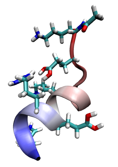
charmm pdbname=cpept < add_h_min.inp > add_h_min.out

Output: cpept_h.pdb, cpept_h.psf and cpept_h.crd. See figure above.

2. Single-temperature CPHMD simulations

With the structure (.pdb or .crd) and .psf files containing dummy hydrogens, we prepare a CHARMM input script for the constant pH Langevin simulation with the GBSW implicit-solvent model at pH 4. CPHMD is currently not implemented with explicit solvent.

charmm < cphmd-cpept.inp > cphmd-cpept.out

Output: /data/*.res, *.dcd, *.eng, *.pdb, and *.lambda

.lambda: lambda values for all titrating sites printed out at specified printing frequency.

3. Replica-exchange CPHMD simulations

REX-CPHMD is the recommended mode for running CPHMD simulations whenever CPUs are available because of the significant improvement in the convergence of the titration property. It is implemented in the MMTSB toolset, and can be invoked using the command, aarex.pl, with the following extra options.

-mdpar param=22x,xpar=par_all22_prot_cmap_phmd.inp,xtop=top_all22_prot_cmap_phmd.inp,

phmdpar=phmd.in,phmdpri=500,phmdph=4.0

The last three options give the parameter file for the titration of model compounds, printing frequency for lambda/x values, and titration pH. We recommend to set the lambda/x printing frequency to be the same as the number of dynamics steps (dynsteps=500).

Type the following command to submit a pbs job for REX-CPHMD simulations of C-peptide at pH 4 with an ionic strength of 150 mM.

qsub rex-cphmd-cpept.pbs

4. Process lambda files and calculate pKa's

From the above REX-CPHMD simulations, you will obtain one lambda file in each replica directory that looks like this.

# ititr 1 2 3 4 5 6 7 8 9
# ires 1 2 2 7 9 9 10 12 12
# itauto 0 3 4 0 3 4 0 1 2
500 0.02 0.99 0.01 0.03 0.01 0.99 0.02 0.02 0.02

Line 1: running number for lambda and x variables
Line 2: corresponding residue number as in the PDB file
Line 3: 0 - single-site titration; 3 4 - carboxyl group; 1 2 - histidine
Line 4 and below: step number, lambda and x values. For example,

0.02 - lambda value for Lys-1
0.99 - lambda value for Glu-2
0.01 - x value for Glu-2
0.03 - lambda value for Lys-7

4.1 Obtain lambda values and unprotonated fractions from REX-CPHMD simulations

Here we introduce several shell and perl scripts to facilitate the tasks.

To extract lambda values for one temperature window:

extractLamb.pl [# replicas] [# rex steps] [lambda printing frq] [# dyna steps] [rex info file] [lambda file]

The rex info file can be created using rexinfo.pl.

The following shell script does both tasks at once (assuming lamb printing and # dyna steps to be 500).

getRexLam.csh [# replicas] [# rex steps] [pH] [rex condition number]

For example, rex-cpept.ph-4/ contains the simulation data for 500 rex steps.

cd rex-cpept.ph-4/cpept.ph-4
../../bin/getRexLam.csh 8 500 4.0 0

Output:

ph-4.ens0-500.lambda (lambda and x values for the 298 K window)

ph-4.0.ens0-500-1-500.sx (fractions of unprotonated/tautomer states)

The .sx file is generated by the Per script, cptSX.pl, which is called at the end of getRexLam.csh.

# ires pH unprot pure mixed
1 1 4.0 0.00 0.97 0.03 --> unprot fraction 0.0 for Lys-1
2 2 4.0 0.53 0.83 0.17 --> unprot fraction 0.53 for Glu-2
3 2 4.0 0.54 0.92 0.08 --> fract of tautomer state 1 is 0.54 for Glu-2
4 7 4.0 0.00 0.98 0.02
5 9 4.0 0.65 0.78 0.22
6 9 4.0 0.54 0.88 0.12
7 10 4.0 0.00 1.00 0.00
8 12 4.0 0.01 0.84 0.16 --> unprot fraction 0.01 for His-12
9 12 4.0 0.58 0.91 0.09 --> fract of HSE tautomer for His-12

We can also use cptSX.pl directly to get S values for certain exchange steps.

cptSX.pl [lambda_file_name] [first exchange step] [last exchange step] [pH]

For example, to generate unprot/tautomer fractions for the last 250 steps:

bin/cptSX.pl ph-4.ens0-500.lambda 251 500 4.0

4.2 Calculate pKa values by fitting to Henderson-Hasselbach (HH) equation.

There are two ways to calculate pKa. If you have one S value on the titration slope, you can get pKa using the S value at one pH by solving the HH equation, S = 1/[1+10^(pka-pH)].

If you have multiple S values obtained at different pH, you can get pKa by fitting the data to the generalized HH equation, S = 1/[1+10^(n*(pka-pH))], where n is the Hill coefficient.

Note: to obtain accurate pKa, it is desirable to have at leat one data point on the titration slope.

A Per script, cptpKa.pl, can be uesd to calculate pKa's for all titrating sites and make titration plots if there are two or more data points.

cptpKa.pl [name] [list of .sx files]

Example with two data points:

bin/cptpKa.pl cpept ph-3.0.ens0-500-1-500.sx ph-4.0.ens0-500-1-500.sx

Output:

cpept.pka (resnumber, pKa, Hill coefficient, fitting correlation coefficient)
cpept-res-*.ps (titration plots for titrating residues)
cpept-res-*.dat (S values for titrating residues)
cpept-res-*.fit (fitting output from xmgrace)

Example with only one data points:

bin/cptpKa.pl ph-4.0.ens0-500-1-500.sx

Output:

ph-4.0.ens0-500-1-500.pka (contains resnumber, pKa, Hill coefficient)

Note, if S is close to 0 or 1, pKa can't be determined. Hence, NA is given in the above file.

5. Derive parameters for model PMF functions

The CPHMD method relies on the calculation of the deprotonation free energy of a titrable site in reference to that of a model compound, which represents an isolated amino acid in solvent and can be constructed using blocking groups, CH3CO-X-NHCH3. We will show how to derive the potential of mean force (PMF) for titrating a model compound.

5.1 Parameters for the model PMF of Lys

Functional form:

Umod = A(sin^2(theta)-B)^2
dUmod/dtheta = 2*A*sin(2*theta)*(sin(theta)^2-B)

First, a parameter file, phmd_blank.in, is prepared. The first line contains the model pKa value and three zero's, which represent the parameter A and B as well as the barrier potential.

Step 1: Build a model compound for Lys

charmm < build-lys.inp

Step 2: Obtain dU/dtheta for a set of theta values

Following shell script can be used to submit the pbs job, rex-phtest1.pbs, with different theta values.

./run-rex-phtest-lys.csh

Each replica directory contains a lambda (dU/dtheta) file that gives the printing frq, theta, and dU/dtheta.

500 1.0000 -3.6955

Step 3: Compile a file, lys.du.dat, which contains the ensemble average of dU/dtheta at different theta values.

The following shell script can be used to calculate the ensemble averages for the above theta values and to compile the averages together into the output file, lys.du.dat.

./bin/getdU.csh

Step 4: Fit the data, lys.du.dat, to the dU/dtheta function, and obtain parameters A and B.

You can use xmgrace to do the fitting. As an example, lys.fit contains the saved fitting data from xmgrace.

5.2 Parameters for the model PMF of Asp

Functional form:

Umod = (R1*sin^4(theta) + R2*sin^2(theta) + R3)*(sin^2(thetax)-R4)^2 + R5*sin^4(theta) + R6*sin^2(theta)

The parameters R1 through R6 are related to the input parameters par1, ..., par6.

Step 1: Build a model compound for Asp.

charmm < build-asp.inp

Step 2: Obtain dU/dtheta for a set of theta and thetax values.

The following shell script can be used to submit the pbs job, rex-phtest2.pbs, with different theta and thetax.

./run-rex-phtest-asp.csh

The lambda file in the replica directories contains theta, dU/dtheta, thetax, and dU/dthetax.

# ititr 1 2
# ires 1 1
# itauto 3 4
500 0.4000 5.0330 0.6000 7.5975

Step 3: Compile files, asp.theta-*.dat and asp.thetax-*.dat.

The following script will do the task.

./bin/getdU2.csh

Step 4: Fit the above data to obtain parameters par1 through par6 (see Umod expression).

In phmd.in, the second tautomer block looks like:

Asp1 (EXPERIMENTAL PK_1/2) A) (B) (BARR)
Asp2 (EXPERIMENTAL PK_1/2) (A) (B) (BARTAU) (A10) (B10)
(par1) (par2) (par3) (par4) (par5) (par6)

We will explain below how to obtain parameters, A, B, A10, B10, and par1 through par6.

4a) At each fixed theta value, obtain parameters for the quadratic function of x,
Umod(x;lambda) = A(lambda)*[x-B(lambda)]^2

Use xmgrace to fit theta-@theta.du.data to f = 2*a0*sin(2*x)*(sin(x)^2-a1)
where @theta = [0.0,0.4,...,1.4], a0 = A(lambda); a1 = B(lambda)

Putting these data together, we get three columns, lambda, A(lambda), and B(lambda):

0.0 -31.7524 0.498452
0.4 -23.3167 0.498176
0.6 -15.402 0.499389
0.7854 -8.57582 0.499863
1.0 -2.98944 0.499987
1.2 -0.630955 0.486581
1.4 -0.0287199 0.517327

Notice, B(lambda) should be very close to 0.5, which is the exact solution for B(lambda). Note, if you specify theta=0.8, the program will generate lambda files with theta of 0.7854, which is pi/4. The same applies to thetax.

4b) At each fixed thetax value, obtain parameters for the quadratic function of lambda,
Umod(lambda;x) = A(x)*[lambda-B(x)]^2

use xmgrace to fit thetax-@thetax.du.data to f = 2*a0*sin(2*x)*(sin(x)^2-a1),

where @thetax = [0.0,0.4,...,1.4,1.57], a0 = A(x); a1 = B(x)

Putting these data together, we get three columns, x, A(x), and B(x).

0.0 -82.9913 0.263723
0.4 -79.3002 0.225235
0.6 -76.7037 0.198332
0.7854 -75.7457 0.187358
1.0 -76.7369 0.200008
1.2 -79.5983 0.229233
1.4 -82.1849 0.254985
1.57 -83.1449 0.263317

4c) Fit functions from a), A(lambda), to the quadratic function: Umod = par1*lambda^2 + par2* lambda + par3

Use xmgrace to fit data A(lambda) to f = a0*sin(x)^4+a1*sin(x)^2+a2, where a0 = par1; a1 = par2; a2 = par3

Find the average of B(lambda) = a0, where a0 = par4

4d) Fit functions from b): A(x) and B(x) to the quadratic function, Umod = par1*x^2 + par2* x + par3

Use xmgrace to fit data A(x) to f = a0*sin(x)^4+a1*sin(x)^2+a2, where a2 = R5

Use xmgrace to fit data B(x) to f = a0*sin(x)^4+a1*sin(x)^2+a2, where a2 = R6

4e) A and B: parameters for titrating one site (not used in the program but still nice to have)
For Asp1: fit thetax-1.57.du.data to f = 2*a0*sin(2*x)*(sin(x)^2-a1), where a0 = A, a1 = B
For Asp2: fit thetax-0.0.du.data to f = 2*a0*sin(2*x)*(sin(x)^2-a1), where a0 = A, a1 = B

4f) A10 and B10: parameters for tautomer interconversion (not used in the program but still nice to have)
Fit theta-0.0.du.data to f = 2*a0*sin(2*x)*(sin(x)^2-a1), where a0 = A10, a1 = B10

5.3 Parameters for the model PMF of His

The parameter file for His looks like this.

HSD (EXPERIMENTAL PK_1/2) A) (B) (BARR)
HSE (EXPERIMENTAL PK_1/2) A) (B) (BARR) A10 B10
0.0 0.0 0.0 0.0 0.0 0.0

We don't need parameters, par1 through par 6. Hence, they are 0.0. We only need three data sets, thetax-1.57.du.data, thetax-0.0.du.data, and theta-1.57.du.data

Step 1: Fit thetax-1.57.du.data to f = 2*a0*sin(2*x)*(sin(x)^2-a1), where a0 = A, a1 = B for HSD

Step 2: Fit thetax-0.0.du.data to f = 2*a0*sin(2*x)*(sin(x)^2-a1), where a0 = A, a1 = B for HSE

Step 3: Fit theta-1.57.du.data to f = 2*a0*sin(2*x)*(sin(x)^2-a1), where a0 = A10, a1 = B10

6. References

1) M. S. Lee, F. R. Salsbury, Jr., and C. L. Brooks, III, Proteins, 2004, 56, pp738.
2) J. Khandogin and C. L. Brooks, III, Biophys. J. 2005, 89, pp141.
3) J. Khandogin and C. L. Brooks, III, Biochemistry 2006, 45, pp9363.